Sensor Eccentricity Calibration
Hi all, I’ve recently managed to implement a ‘Sensor Eccentricity Calibration’ for SimpleFoc with the help of Richard. The calibration is based on the blog post from Ben Katz (BuildIts in Progress: Encoder Autocalibration for Brushless Motors: Offset and Eccentricity).
So, what is the goal of this calibration? When you mount your (magnetic) sensor on your frame or motor, there will always be a slight misalignment between magnet and sensor (measurement system). This misalignment between center of rotation and the center of the sensor is called the eccentricity error.
As a result your measurement system output is non-linear with respect to the rotor of the motor. This will cause an error with respect to the ideal torque you attempt to create with the I_q vector as function of the position. You could interpret this as a disturbance on your control loop which you want to minimize for optimal performance. This calibration compensates the sensor reading in a feed forward fashion such that your performance improves.
disclaimer: I’ve not peer reviewed this content so it may not be 100% accurate. I want to post it anyway so people may continue the work or want to test it already (see final chapter). I’m away from SimpleFoc for some time because my son was born last week :).
What does the calibration do?
- Find the direction of sensor.
- Move open loop a mechanical 2PI positive rotation (trace sensor angle & electrical angle) and calculate the difference.
- Move open loop a mechanical 2PI negative rotation (trace sensor angle & electrical angle) and calculate the difference.
- Store the average electrical angle offset
- Post process the data (from forward/backward rotation) to find the error between sensor angle and electrical angle.
- Build the eccentricity LUT (Look Up Table).
- Save this LUT to compensate your calibrated sensor output.
What is the output of the calibration?
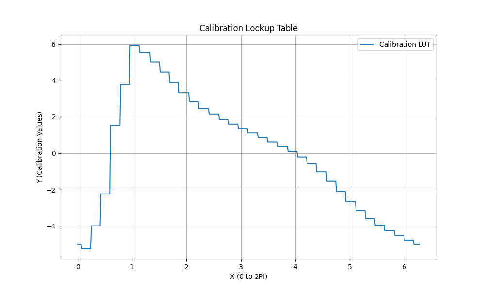
The LUT represents the amount of radians the sensor is wrong with respect to the actual electrical angle. The CalibratedSensor class will read the uncalibrated sensor angle and adds the (interpolated) offset it gets from the LUT. Note that this is a relative measurement between sensor angle and electrical angle. This calibration assumes the electrical angle to be the reference because we want to compensate the sensor towards the correct electrical angle.
This error data is filtered as implemented by Ben Katz and removes the error caused by cogging, which is unrelated to the eccentricity. More details can be found in his blog post.
In my example the peak-to-peak error is around 0.12 rad. However, since this motor has seven pole pairs, the error it makes during commutation is 7x0.12 = 0.84 rad in electrical angle, which is significant. As you can imagine this becomes more problematic if you have high pole pair motors or if your sensor is mounted more eccentric since the commutation error is NPP*Eccentricity Error. Disclaimer: the performance increase is not so easily observable if you have a well aligned sensor and a low pole pair motor.

Figure 1 Eccentricty error (Look up Table)
What is the impact on the actual torque output?
In the graph below I visualize the impact of the position dependent measurement error on your actual torque output. In the top graph the optimal FOC output for the three phases is represented. In the second graph I plot the eccentricity error as discussed in the previous section.
In the bottom two plots you see the impact of this eccentricity on the actual torque that is generated. In my case, where I deliberately mounted the sensor with an offset of 0.5 mm, the efficiency will drop down locally to below 90%. Also important to understand is that this disturbance is position dependent and as you will rotate faster, the disturbance will become more high frequent and it will become more troublesome for your feedback controller to compensate. Therefore, you want a known an error like this in advance such that we can compensate it in a feedforward fashion.

Figure 2 Simulated Torque Actual versus Ideal
What is the result of the calibration on the actual velocity for a Torque Control Example?
I’ve tried to visualize the impact of this calibration with a Torque control example where the control loop is trying to keep the voltage constant. In a perfect system, a constant voltage would result in a constant velocity.
As you can see in the graph below the disturbance (eccentricity) is mostly compensated for by our calibrated sensor class. As the target voltage increases and thus the velocity, the disturbance impact becomes larger (it becomes more high frequent). After this calibration the velocity becomes ‘very’ constant (red) as compared to a non-calibrated system (blue).
Table 1: Calibration Performance 2V
| Test | Average Velocity | Standard Deviation |
|---|---|---|
| Uncalibrated Sensor Target 2V | 38.22 | 6.71 rad/s |
| Calibrated Sensor Target 2V | 50.09 | 0.62 rad/s |

Figure 3 Calibrated and Uncalibrated Velocity 2V
Table 2: Calibration Performance 5V
| Test | Average Velocity | Standard Deviation |
|---|---|---|
| Uncalibrated Sensor Target 5V | 73.14 rad/s | 9.23 rad/s |
| Calibrated Sensor Target 5V | 78.78 rad/s | 1.34 rad/s |

Figure 4 Calibrated and Uncalibrated Velocity 5V
Table 3: Calibration Performance 10V
| Test | Average Velocity | Standard Deviation |
|---|---|---|
| Uncalibrated Sensor Target 10V | 87.47 rad/s | 12.58 rad/s |
| Calibrated Sensor Target 10V | 94.85 rad/s | 1.86 rad/s |

Figure 5 Calibrated and Uncalibrated Velocity10V
Sensor,CalibratedSensor,shaft_velocity?
Some work yet to be done is to quantify the improvement on actual achieved velocity. You can see that the shaft velocity improves most and that there is still some variation in the uncalibrated sensor output. Note that the spikes in the calibrated velocity are likely a bug with the getVelocity() function being called twice.
Both figures are with a target velocity of 5V.
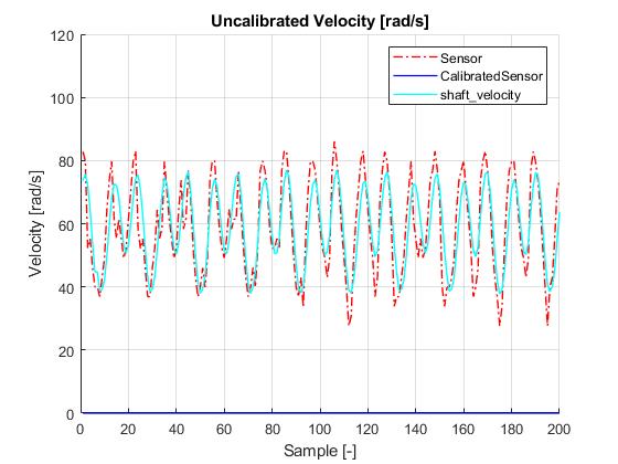
Figure 6 Uncalibrated Velocity 5V shaft_velocity and sensor output
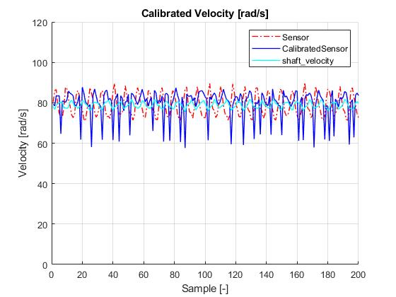
Figure 7 Calibrated Velocity 5V shaft_velocity, sensor and CalibratedSensor output
Video’s
First of all, if you sensor is well aligned and you have a low pole pair motor you likely will not notice the improvement that easily. Anyway, two video’s with and without calibration.
Uncalibrated

Uncalibrated Phase Voltage

Calibrated

Calibrated Phase Voltage

How can I test this code?
It is a pretty raw version of the code and not optimized for memory/performance. So it should likely be improved in the future.
All you need to add to your code is the following. Instantiate the CalibratedSensor class directly after your normal sensor class. In the setup you choose your open loop voltage for this calibration (don’t start too high) and you call the calibration. After the calibration you link the sensor to your motor and you are ready to roll.
I’ve tested it with both the AS5074 and AS5600 with different boards (STM446RE/Arduino) and different drivers (DRV8302 and SimpleFocShield v2)

The Calibration will be made part of the dev branch in the nearby future and can be found here:
An example can be taken from here:
Until it is available you in the dev branch you can get it here: